Censoring and Nonparametric Methods

Coding Review

Setup: R Packages

Key Packages

For Censored Regression:

AER::tobit(): Tobit estimation (censored regression)
quantreg::crq(): CLAD estimation (censored quantile regression)

For Nonparametric Methods:

np::npreg(): Nonparametric regression (Nadaraya-Watson, local linear)
density(): Kernel density estimation (base R)

Censoring and Tobit

Exercise 1: Understanding the Three CEFs

Before fitting any model, it helps to visualize what the three conditional expectations \(m^*(x)\), \(m(x)\), and \(m^\#(x)\) actually look like. Here we simulate data from a known Tobit model and compare them.

Exercise 2: Comparing OLS, Truncated OLS, and Tobit

Now fit all three estimators and compare their coefficients to the true \(\beta = 1.5\).

model_ols <- lm(y ~ x)
model_trunc <- lm(y ~ x, subset = y > 0)
model_tobit <- tobit(y ~ x, left = 0, data = data.frame(y = y, x = x))

cat("True beta: 1.5\n\n")
cat("OLS (all data):      ", round(coef(model_ols)["x"], 3), "\n")
cat("OLS (truncated):     ", round(coef(model_trunc)["x"], 3), "\n")
cat("Tobit:               ", round(coef(model_tobit)["x"], 3), "\n")
cat("\nCensoring rate:", round(mean(y == 0), 3))

Interpretation

OLS on all data underestimates \(\beta\): the zeros drag the slope toward zero. Greene’s formula \(E[\hat{\beta}_{OLS}] \approx \beta(1-\pi)\) gives a rough prediction of this bias.
OLS on truncated data overestimates \(\beta\): dropping zeros leaves only the high-\(y\) observations in the sample. For high-\(x\) this is most of them, but for low-\(x\) you are left with only the unlucky positive draws, biasing the slope upward.
Tobit recovers \(\beta \approx 1.5\) because it correctly models both the probability of being zero and the magnitude when positive.

The direction of bias for truncated OLS (upward) vs all-data OLS (downward) is a key conceptual point from the lectures.

Exercise 3: Marginal Effects

The Tobit coefficient is not the marginal effect on observed \(Y\). Calculate both marginal effects.

b_hat <- coef(model_tobit)["x"]
sigma_hat <- model_tobit$scale
x_mean <- mean(x)

xb_over_s <- (b_hat * x_mean) / sigma_hat

# Marginal effect on E[Y | X]
me_full <- pnorm(xb_over_s) * b_hat

# Marginal effect on E[Y | X, Y>0]
inv_mills <- dnorm(xb_over_s) / pnorm(xb_over_s)
me_pos <- b_hat * (1 - inv_mills * (xb_over_s + inv_mills))

cat("Tobit coefficient:  ", round(b_hat, 3), "\n")
cat("ME on E[Y|X]:       ", round(me_full, 3), "\n")
cat("ME on E[Y|X,Y>0]:   ", round(me_pos, 3), "\n")

Interpretation

The Tobit coefficient represents the effect of \(X\) on the latent variable \(Y^*\). The marginal effect on observed \(Y\) is smaller, scaled down by \(\Phi(X'\beta/\sigma)\) – the probability of being uncensored at that value of \(X\).

Intuitively: a 1-unit increase in \(X\) shifts the latent demand up by \(\beta\). But for people already at zero who are close to the margin, some of them now become positive. For people well below zero, they are still zero. The probability \(\Phi(X'\beta/\sigma)\) captures what fraction of the population is “responsive” to \(X\).

CLAD Estimation

Exercise 4: Tobit vs CLAD under Misspecification

CLAD is more robust than Tobit when the error distribution is not normal. Here we compare them under a fat-tailed error distribution.

library(quantreg)

set.seed(123)
n <- 800
x2 <- runif(n, -2, 2)
beta_true <- 2

e <- rt(n, df = 3)
y_star2 <- beta_true * x2 + e
y2 <- pmax(y_star2, 0)

model_tobit2 <- tobit(y2 ~ x2, left = 0)
model_clad <- crq(Surv(y2, y2 > 0, type = "left") ~ x2, tau = 0.5, method = "Powell")

cat("True beta: ", beta_true, "\n")
cat("Tobit:     ", round(coef(model_tobit2)["x2"], 3), "\n")
cat("CLAD:      ", round(coef(model_clad), 3), "\n")

Interpretation

With fat-tailed errors, Tobit’s normality assumption is violated. The heavy tails inflate the variance of extreme observations, distorting the MLE. CLAD, which relies only on the median having the right location, is more robust and should be closer to the true \(\beta = 2\).

The tradeoff: CLAD is harder to optimize (no guaranteed global minimum), and it estimates the median rather than the mean, which may not be the quantity of interest.

Kernel Density Estimation

Exercise 5: Bandwidth Sensitivity

The bandwidth \(h\) is the most important choice in kernel density estimation. Here we explore how it affects the estimate.

Interpretation

Small bandwidth (undersmoothing): The estimate is noisy and wiggly. It overfits to random variation in the data.
Large bandwidth (oversmoothing): The estimate is too smooth. The bimodal structure is completely hidden.
Medium bandwidth: The two modes are visible and the estimate looks reasonable.

This is the bias-variance tradeoff from the lecture notes: AIMSE = bias term (increases with \(h\)) + variance term (decreases with \(h\)).

Exercise 6: Silverman’s Rule and Cross-Validation

Compare automatic bandwidth selection methods.

Interpretation

For this bimodal distribution, cross-validation selects a smaller bandwidth than Silverman’s rule. This makes sense: Silverman’s rule is derived assuming the data are normally distributed. For a bimodal distribution, the normal assumption leads to oversmoothing (the rule “sees” a wide spread in the data and infers a large bandwidth), but what it is really seeing is the separation between two modes.

Cross-validation is preferred for multimodal or asymmetric distributions. Silverman’s rule is a good default for approximately normal data.

Nonparametric Regression

Exercise 7: Nadaraya-Watson vs Local Linear

Implement both estimators from scratch using base R – no packages needed. This mirrors equations (19.2) and (19.4) directly from the lecture notes.

The Nadaraya-Watson estimator at a single point \(x_0\) is:

\[\hat{m}^{nw}(x_0) = \frac{\sum_i K\!\left(\frac{X_i - x_0}{h}\right) Y_i}{\sum_i K\!\left(\frac{X_i - x_0}{h}\right)}\]

The local linear estimator fits a weighted least squares regression \(Y_i \sim \alpha + \beta(X_i - x_0)\) with kernel weights, and takes \(\hat{\alpha}\) as the estimate of \(m(x_0)\).

nw_at <- function(x0, x, y, h) {
  w <- dnorm((x - x0) / h)
  sum(w * y) / sum(w)
}

ll_at <- function(x0, x, y, h) {
  w     <- dnorm((x - x0) / h)
  X_loc <- cbind(1, x - x0)
  fit   <- lm.wfit(X_loc, y, w)
  fit$coefficients[1]
}

Interpretation

Both estimators track \(m(x) = \sin(2x) + x/2\) well in the interior of the data, but differences emerge near the boundaries (around \(\pm\pi\)):

The Nadaraya-Watson estimator is biased at the boundary because only observations on one side are available. The neighborhood is asymmetric, and the density gradient term \((f'(x)/f(x))m'(x)\) in the bias formula is large here – the one-sided average pulls the estimate away from the true function.

The local linear estimator handles the boundary better. By fitting a line rather than a constant in each neighborhood, it can extrapolate the local slope into the region where data is sparse. The slope estimate compensates for the asymmetric neighborhood, eliminating the density gradient bias term entirely.

This boundary behavior is the main practical reason Hansen recommends local linear over Nadaraya-Watson, and why you can see the difference most clearly at the edges of the plot.

Verification with np package (static output):

The chunk below runs the same data through np::npreg() with the same fixed bandwidth to confirm the manual implementations match.

library(np)
library(tidyr)
library(ggplot2)

set.seed(7)
n <- 300
h <- 0.4

x_np <- runif(n, -pi, pi)
y_np <- sin(2 * x_np) + x_np / 2 + rnorm(n, 0, 0.5)

x_grid_np <- seq(-pi, pi, length.out = 100)
m_true    <- sin(2 * x_grid_np) + x_grid_np / 2

# Manual implementations (same as exercise)
nw_at <- function(x0, x, y, h) {
  w <- dnorm((x - x0) / h); sum(w * y) / sum(w)
}
ll_at <- function(x0, x, y, h) {
  w <- dnorm((x - x0) / h)
  fit <- lm.wfit(cbind(1, x - x0), y, w)
  fit$coefficients[1]
}
m_nw_manual <- sapply(x_grid_np, nw_at, x = x_np, y = y_np, h = h)
m_ll_manual <- sapply(x_grid_np, ll_at, x = x_np, y = y_np, h = h)

# np package with same fixed bandwidth
bw_nw <- npregbw(y_np ~ x_np, regtype = "lc", bws = h, bandwidth.compute = FALSE)
bw_ll <- npregbw(y_np ~ x_np, regtype = "ll", bws = h, bandwidth.compute = FALSE)
m_nw_np <- npreg(bw_nw, exdat = x_grid_np)$mean
m_ll_np <- npreg(bw_ll, exdat = x_grid_np)$mean

# Plot comparing manual vs np
# Prepare data for plotting
df_nw <- data.frame(
  x = x_grid_np,
  Manual = m_nw_manual,
  np_pkg = m_nw_np
) %>%
  pivot_longer(-x, names_to = "Method", values_to = "Estimate")

df_ll <- data.frame(
  x = x_grid_np,
  Manual = m_ll_manual,
  np_pkg = m_ll_np
) %>%
  pivot_longer(-x, names_to = "Method", values_to = "Estimate")

# Nadaraya-Watson plot
p_nw <- ggplot(df_nw, aes(x = x, y = Estimate, color = Method, linetype = Method)) +
  geom_line(size = 1) +
  labs(title = "NW: Manual vs np", x = "x", y = "m(x)") +
  scale_color_manual(values = c("firebrick", "black")) +
  theme_bw()

# Local Linear plot
p_ll <- ggplot(df_ll, aes(x = x, y = Estimate, color = Method, linetype = Method)) +
  geom_line(size = 1) +
  labs(title = "LL: Manual vs np", x = "x", y = "m(x)") +
  scale_color_manual(values = c("steelblue", "black")) +
  theme_bw()

print(p_nw)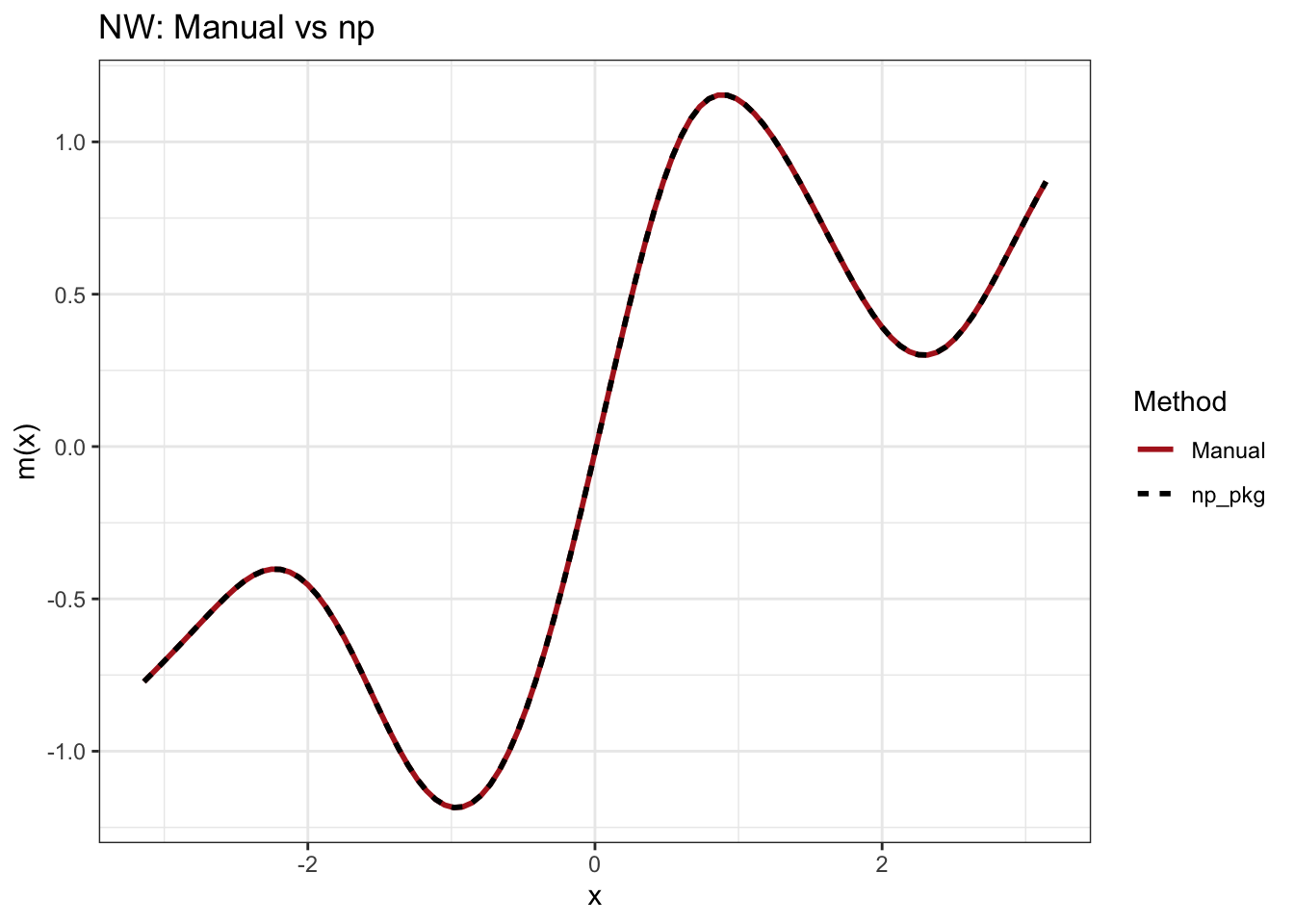

print(p_ll)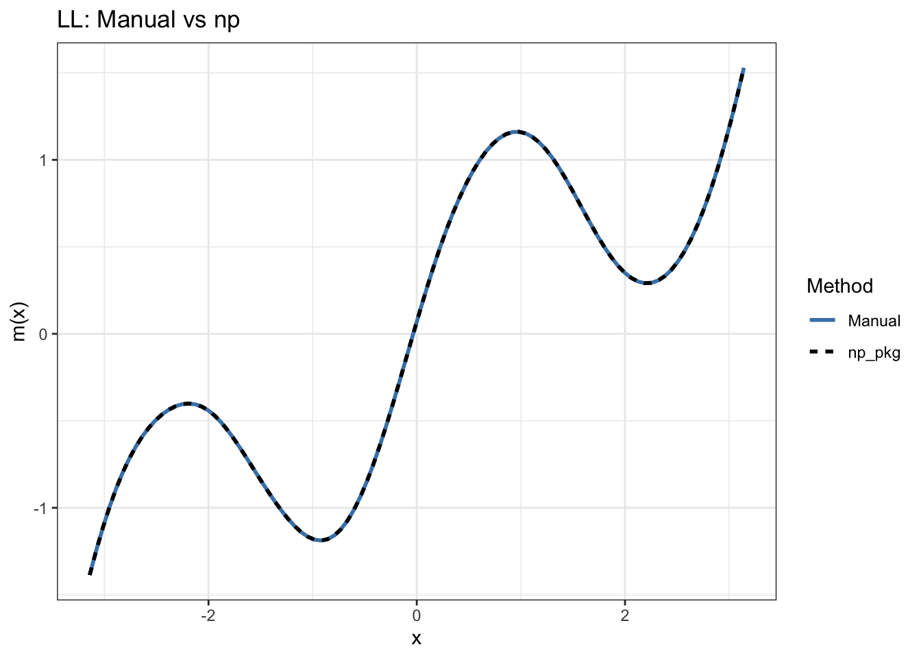

Max |manual NW - np NW|: 0 Max |manual LL - np LL|: 0

Exercise 8: Cross-Validation Bandwidth

Visualize the CV criterion as a function of \(h\) to understand what cross-validation is doing.

h_grid <- seq(0.05, 1.5, by = 0.05)
cv_vals <- numeric(length(h_grid))

for (j in seq_along(h_grid)) {
  h <- h_grid[j]
  loo_errors <- numeric(n_cv)
  for (i in 1:n_cv) {
    dists <- (x_cv[-i] - x_cv[i]) / h
    weights <- dnorm(dists)
    if (sum(weights) > 0) {
      m_loo <- sum(weights * y_cv[-i]) / sum(weights)
    } else {
      m_loo <- mean(y_cv[-i])
    }
    loo_errors[i] <- (y_cv[i] - m_loo)^2
  }
  cv_vals[j] <- mean(loo_errors)
}
h_opt <- h_grid[which.min(cv_vals)]

Interpretation

The CV curve is U-shaped:

Left side (small \(h\)): Each point is estimated using very few neighbors. The fit is noisy and the leave-one-out errors are large because the estimate at each \(x_i\) is heavily influenced by just a handful of points – removing one observation changes the estimate substantially.
Right side (large \(h\)): Each point is estimated using the whole dataset. This is essentially fitting a constant. The systematic bias (underfitting a curved function) dominates.
Minimum: The CV-optimal bandwidth balances these two sources of error.

This is the empirical counterpart of minimizing AIMSE = bias\(^2\) + variance.

Summary

Method	Estimand	Key assumption	What goes wrong if violated
OLS on \(Y\)	\(E[Y^* \mid X]\)	No censoring	Attenuation bias toward zero
OLS on \(Y^\#\)	\(E[Y^\# \mid X]\)	Random truncation	Upward bias
Tobit	\(E[Y^* \mid X]\)	Normality, homoskedasticity	Inconsistent
CLAD	\(\text{Med}[Y^* \mid X]\)	Symmetric median at zero	Local optima in estimation
Kernel density	\(f(x)\)	Smoothness of \(f\)	Larger bandwidth needed
Nadaraya-Watson	\(E[Y \mid X=x]\)	Smoothness of \(m(x)\), \(f(x)\)	Boundary bias
Local linear	\(E[Y \mid X=x]\)	Smoothness of \(m(x)\)	Slightly wider confidence bands

Key practical takeaways:

Always check the censoring rate before choosing an estimator. If it is very high (\(> 80\%\)), estimates of any kind are fragile.
Report Tobit and CLAD side by side. Large disagreements suggest distributional misspecification.
For kernel regression, the bandwidth matters far more than the choice of kernel. Always try multiple bandwidths and use cross-validation or a rule of thumb.
Local linear is strictly preferred to Nadaraya-Watson in practice.